Numerical Results
Solutions
In order to test our method, we will construct exact solutions to Maxwell’s Equations that satisfy our assumptions. Namely, we wish to construct solution that satisfies the divergence free constraint that is, at least numerically, compactly supported.
2D solution
We use the solution to the transverse magnetic problem given by
where \(\phi\) is a solution of the scalar wave equation produced by a point source with the time amplitude \(e^{-125(t + .475)^2}\). This solution is computed numerically to at least 10 digits. An end-point corrected quadrature scheme to deal with the singularity in the Green’s function for the wave equation in 2D. Boundary conditions are satisfied using the method of images.
Derivation of a 3D solution
If we choose \(\mathbf{W}\) to be a solution to the wave equation with speed \(c = \frac{1}{\sqrt{\varepsilon \mu}}\), then we can ensure that our solution is divergence free by defining
Then, we can define
Since \(\mathbf{W}\) satisfies the wave equation by assumption, we have
therefore,
Using the vector identity \(\nabla^2 \mathbf{A} = \nabla (\nabla \cdot \mathbf{A}) - \nabla \times (\nabla \times \mathbf{A})\), we have
Similarly, we have
So we see Maxwell’s equations are satisfied. Furthermore, we can guarantee that our solution is compactly supported, as desired, with a careful choice of \(\mathbf{W}\).
Satisfying Boundary Conditions
We can satisfy boundary conditions using the method of images. To illustrate this, we want consider the 3D waveguide problem in the domain
with PEC boundary conditions at \(y = 0\), \(y = a\), \(z = 0\), and \(z = b\).
In order to satisfy the PEC boundary conditions at \(z=0\) and \(z=z_{max}\), we have
therefore, we require \(w_1\) to be even in \(z\), \(w_2\) to be even in z, and \(w_3\) to be odd in \(z\). Similarly, we have
for the PEC boundary conditions at \(y=0\) and \(y=y_{max}\), so we will require \(w_1\) to be even in \(y\), \(w_2\) to be odd in \(y\), and \(w_3\) to be even in \(y\).
Finally, given a source location we can enforce these conditions by adding images of the appropriate source components (with the appropriate signs) which have been reflected across the boundaries.
Implementation Detail
In the implementation of out test problems, we choose all three components of \(\mathbf{W}\) to be
where \(r = \sqrt{(x_1-x_{1_{src}})^2 + (x_2-x_{2_{src}})^2 +(x_3-x_{3_{src}})^2}\) and \(\tau > 0\). It is easy to verify that this is a point source solution of the wave equation. Noting that \(e^{-36} \approx 2.3195 \cdot 10^{-16}\), we can derive approximate bounds for the minimum and maximum distances the image sources can be from a given point and contribute to the solution at that point. Based on the chosen form, numerically, we will see no contributions if the following is true
This implies that we only need to consider the image sources in the region given by
In practice, we first generate possible source locations in the looser bounds given by inscribing a box in the lower bound and inscribing the upper bound in a box. After generating the possible locations, we then check these possibilities against the bound and only keep the sources that contribute.
When using this routine to generate initial conditions for simulations using the Yee scheme, we compute the curl numerically using the same discrete curl operator that is used in the Yee updates. This gives us initial conditions that are numerically divergence free for the simulations. Furthermore, comparing the initial conditions computed using the discrete and analytical divergence operators gives us a good approximation of the discretization error we expect in the simulations.
Free Space Transverse Magnetic Problem
We simulated the free space transverse magnetic problem given by
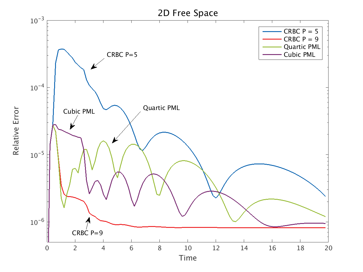
where \(\phi\) is a solution of the scalar wave equation produced by a point source centered at \((0, 0)\) with the time amplitude \(e^{-125(t + .475)^2}\). The CRBC/DAB boundaries were placed at \(x=\pm 1\) and \(y=\pm 1\). For this test, we used a grid size of \(3000 \times 3000\) in the \(E_z\) component. The errors reported are relative to the initial condition and are given by the following formula
For comparison purposes we also ran the simulation using a convolution PML (CPML) with suggested parameters from the literature. We note that it is likely possible to find a set of parameters for the CPML that will perform better than those presented for this problem. For these tests, we used a PML 10 Yee cells thick and tried cubic and quartic ramping functions.
In the following plot showing behavior at short times, we can see that it is possible to get comparable results for both the CRBC/DAB boundaries and the CPML boundaries, depending on the chosen parameters. In the following plot showing behavior at long times, it appears that the both boundaries have practically identical behaviors.
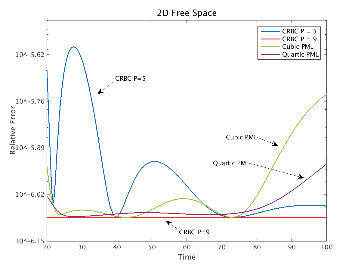
Finally, the following table summarizes the simulation results.
Grid |
DOFs |
BC |
Max Rel Err |
|---|---|---|---|
\(3000 \times 3000\) |
\(2.72 \times 10^{7}\) |
CRBC P = 5 |
\(3.73 \times 10^{-4}\) |
\(3000 \times 3000\) |
\(2.73 \times 10^{7}\) |
CRBC P = 9 |
\(2.76 \times 10^{-5}\) |
\(3020 \times 3020\) |
\(2.77 \times 10^{7}\) |
Cubic PML |
\(2.76 \times 10^{-5}\) |
\(3020 \times 3020\) |
\(2.77 \times 10^{7}\) |
Quartic PML |
\(2.80 \times 10^{-5}\) |
Transverse Magnetic in a Wave Guide
To test these boundary conditions, we again simulated the transverse magnetic problem given by
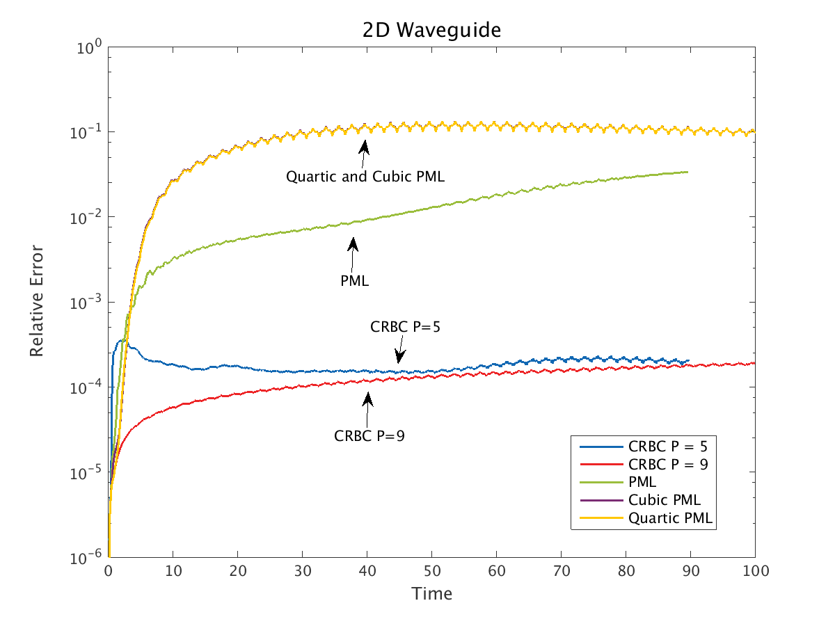
where \(\phi\) is a solution of the scalar wave equation satisfying zero Dirichlet (PEC) boundary conditions at \(y=0\) and \(y=1\) produced by a point source centered at \((0, 0.1)\) with a time amplitude \(e^{-125(t + .475)^2 }\). The CRBC/DAB and PML boundaries were placed at \(x=\pm 1\) and the grid was \(6000 \times 3000\) in the \(E_z\) component.
The errors reported are relative to the initial condition and are given by the following formula
For comparison purposes we also ran the simulation using a convolution PML (CPML) with suggested parameters from the literature. We note that it is likely possible to find a set of parameters for the CPML that will perform better than those presented for this problem. For these tests, we used a PML 10 Yee cells thick and tried cubic and quartic ramping functions. The final run labeled “PML” corresponds to choosing the PML parameter \(\sigma_{max}\) to be approximately twice as large as suggested with quartic ramping.
In 2D waveguide plot, we see that the DAB boundaries perform much better than the PML. Furthermore, we see that suggested parameter values for the PML sometimes perform poorly.
Finally, the following table summarizes the simulation results.
Grid |
DOFs |
BC |
Max Rel Err |
|---|---|---|---|
\(6000 \times 3000\) |
\(6.01 \times 10^{7}\) |
CRBC P = 5 |
\(3.52 \times 10^{-4}\) |
\(6000 \times 3000\) |
\(6.02 \times 10^{7}\) |
CRBC P = 9 |
\(1.94 \times 10^{-4}\) |
\(6020 \times 3000\) |
\(6.04 \times 10^{7}\) |
PML |
\(3.37 \times 10^{-2}\) |
\(6020 \times 3000\) |
\(6.04 \times 10^{7}\) |
Cubic PML |
\(1.34 \times 10^{-1}\) |
\(6020 \times 3000\) |
\(6.04 \times 10^{7}\) |
Quartic PML |
\(1.33 \times 10^{-1}\) |
3D Wave Guide
Using a solution generated from a point source solution to the wave equation with a Gaussian time amplitude as described in the solutions section, we have tested our implementation of the DAB boundaries on the domain \([0,1.6] \times [0,1.6] \times [0,1.6]\) with DAB boundaries at \(x = 0\) and \(x =1.6\) and PEC boundaries elsewhere. The source location was \(( 0.8, 0.8, 0.8)\) and we used the solution parameters \(\tau = 0.39\) and \(\gamma = 130\) with material parameters \(\epsilon = 0.8\) and \(\mu = 1.25\). The simulations were run with the CRBC parameter \(P = 3\) and \(P = 5\) on a grid with \(n\) Yee cells in each spatial direction.
For the \(P = 3\) case, we can see that we stay below the reflection coefficient for about a third of the simulation in the 3D waveguide plot (P = 3). For the \(P = 5\) case, we see approximately the same behavior as the \(P = 3\) case in the 3D waveguide plot (P = 5). This behavior indicates that the discretization error is dominant in most cases and we believe the error at later times can be explained by numerical dispersion.
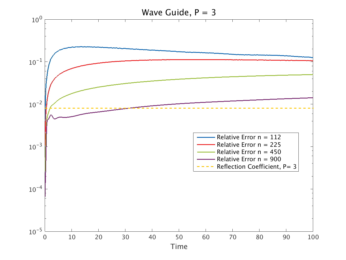
3D waveguide plot (P = 3)
Relative Error for a 3D wave guide simulation and and the expected reflection coefficients.
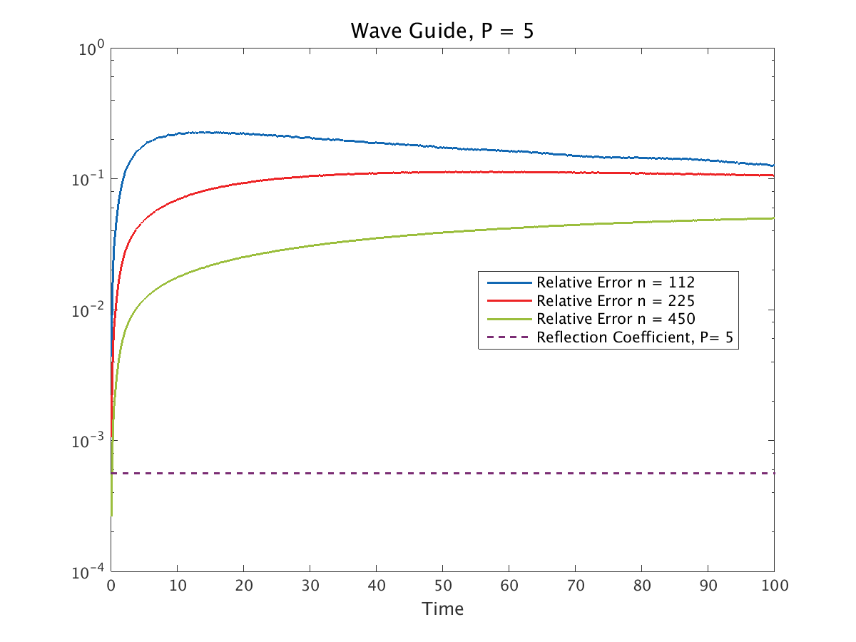
3D waveguide plot (P = 5)
Relative Error for a 3D wave guide simulation and and the expected reflection coefficients.
Parallel Plates
Using a solution generated from a point source solution to the wave equation with a Gaussian time amplitude as described in the solutions section, we have tested our implementation of the DAB boundaries on the domain \([0,1.6] \times [0,1.6] \times [0,1.6]\) with PEC boundaries at \(z = 0\) and \(z =1.6\) and DAB boundaries elsewhere. The source location was \(( 0.8, 0.8, 0.8)\) and we used the solution parameters \(\tau = 0.39\) and \(\gamma = 130\) with material parameters \(\epsilon = 0.8\) and \(\mu = 1.25\). The simulations were run with the CRBC parameter \(P = 3\) and \(P = 5\) on a grid with \(n\) Yee cells in each spatial direction.
Similar to the wave guide case, for the \(P = 3\) case, we can see that we stay below the reflection coefficient when using a sufficiently refined grid in the 3D parallel plates plot (P = 3). For the \(P = 5\) case, we again see approximately the same behavior as the \(P = 3\) case in the 3D parallel plates plot (P = 5). This behavior indicates that the discretization error is dominant in most cases. Compared to the wave guide example, the better long time error behavior is due to the fact that more energy leaves the computational domain and the numerical dispersion has less effect.
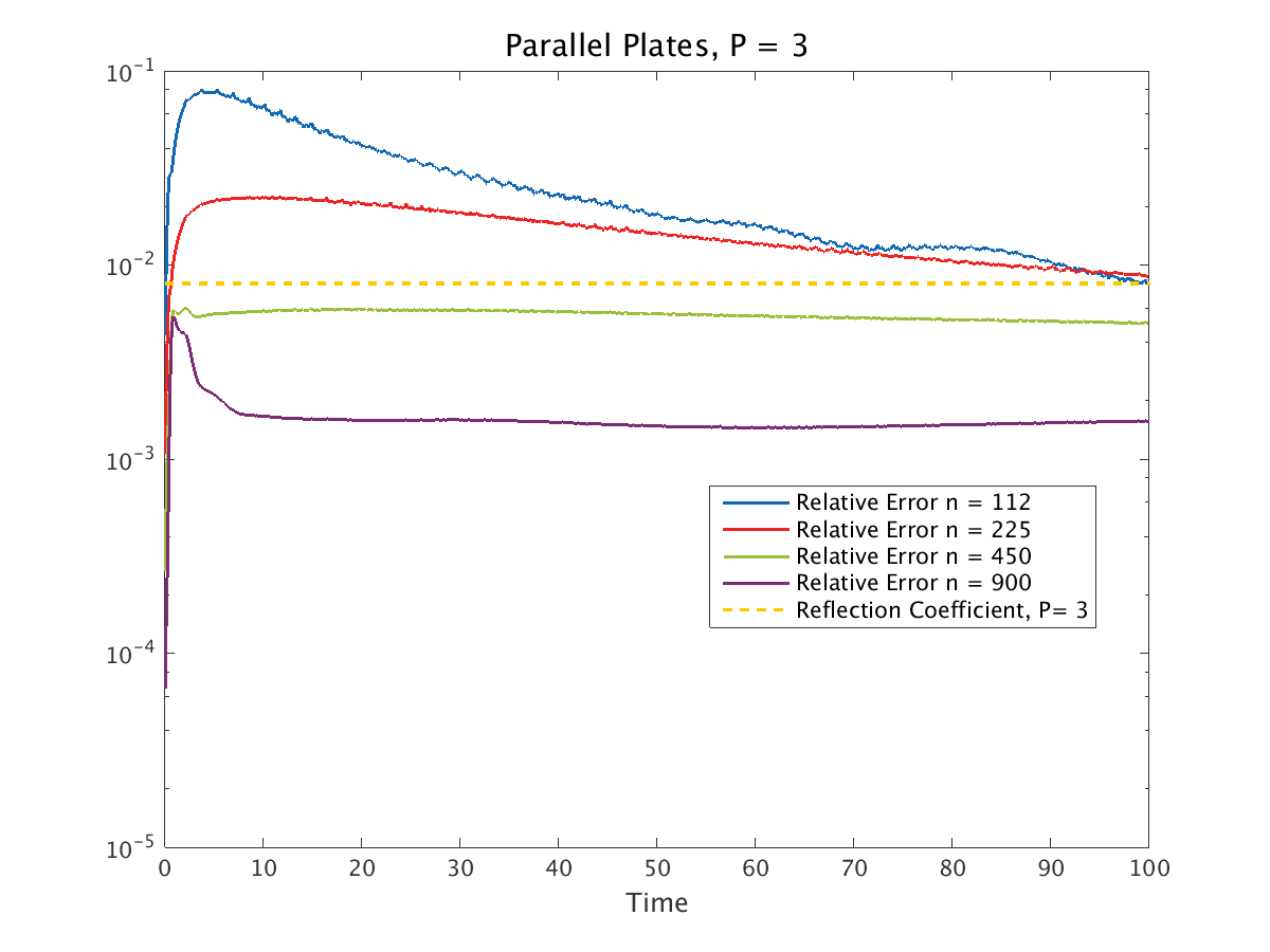
3D parallel plates plot (P = 3)
Relative Error for a 3D parallel plate simulation and and the expected reflection coefficients.
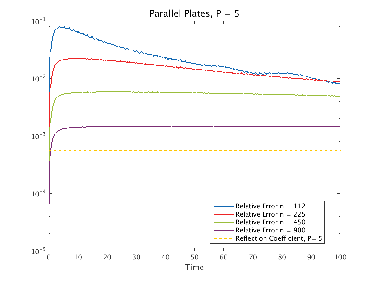
3D parallel plates plot (P = 5)
Relative Error for a 3D parallel plate simulation and and the expected reflection coefficients.
Free Space
Again, using a solution generated from a point source solution to the wave equation with a Gaussian time amplitude as described in the solutions section, we have tested our implementation of the DAB boundaries on the domain \([0,1.6] \times [0,1.6] \times [0,1.6]\) with DAB boundaries one all faces. The source location was \(( 0.8, 0.8, 0.8)\) and we used the solution parameters \(\tau = 0.39\) and \(\gamma = 130\) with material parameters \(\epsilon = 0.8\) and \(\mu = 1.25\). The simulations were run with the CRBC parameter \(P = 3\) and \(P = 5\) on a grid with \(n\) Yee cells in each spatial direction.
For the free space simulation, we see that we are able to meet the error bounds provided by the expected reflection coefficients up to \(P=7\). Looking at the 3D free space plot (P = 3), we can see that relative error “steps” down in a more or less regular pattern. This happens because some amount of the wave front erroneously reflects off of the boundary and a large portion of this reflected wave is absorbed when it reaches the opposite boundary. We can see this behavior in the 3D free space plot (P = 5) and the 3D free space plot (P = 7) and we note that in all of these cases the reflection coefficient is a good predictor of where this behavior occurs, as expected. In the 3D free space plot (P = 9), we see that the discretization error dominates and we never reach the reflection coefficient. Finally, in the 3D free space plot (long time, P = 7), we show that relative error remains constant over a long time (this occurs for all of the simulations, but we have omitted the plots). In these simulations, we believe the long time error are on the order of discretization error.
These plots also demonstrate that choosing the a tolerance so that a reflection coefficient is approximately equal to the discretization error is a good choice. For instance, we can see that \(P=5\) is a good choice for \(n=112\) and \(p=7\) is a good choice for \(n=450\).
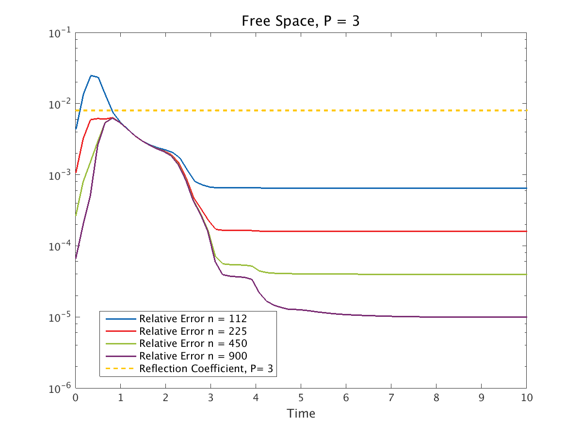
3D free space plot (P = 3)
Relative Error for a 3D free space simulation and the expected reflection coefficients.
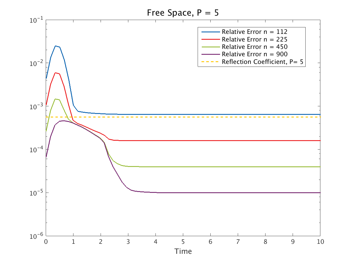
3D free space plot (P = 5)
Relative Error for a 3D free space simulation and the expected reflection coefficients.
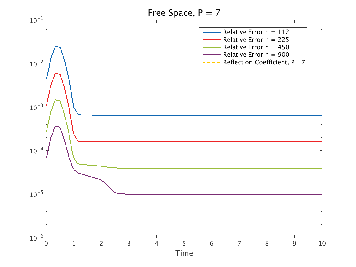
3D free space plot (P = 7)
Relative Error for a 3D free space simulation and the expected reflection coefficients.
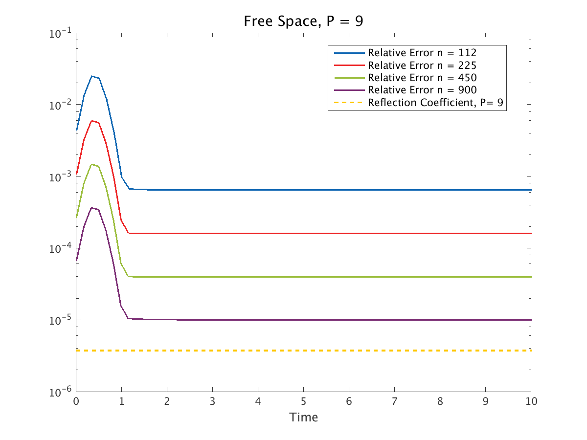
3D free space plot (P = 9)
Relative Error for a 3D free space simulation and the expected reflection coefficients.
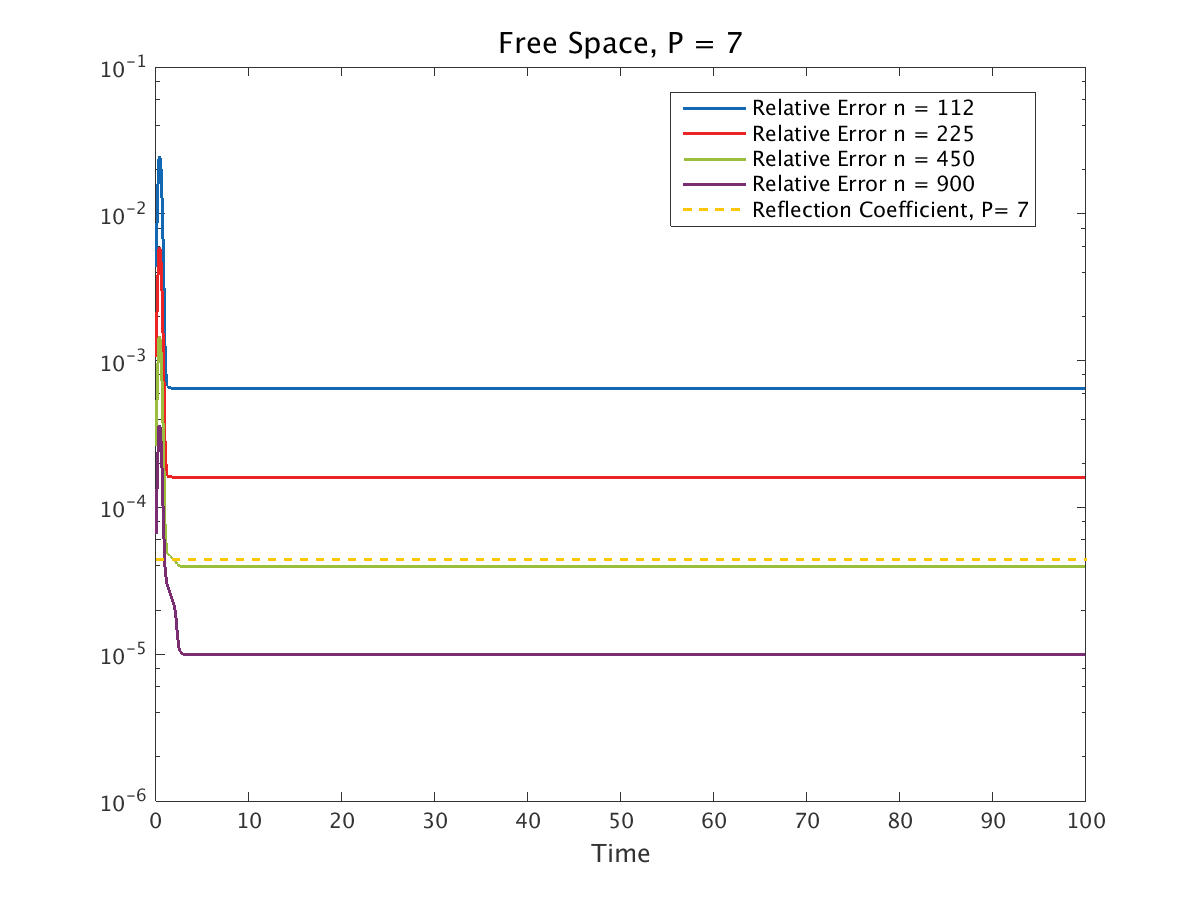
3D free space plot (long time, P = 7)
Relative Error for a 3D free space simulation and the expected reflection coefficients.